Linear model analysis
# import relevant module
import openturns as ot
import otpod
# enable display figure in notebook
%matplotlib inline
Generate data
N = 100
ot.RandomGenerator.SetSeed(123456)
defectDist = ot.Uniform(0.1, 0.6)
# normal epsilon distribution
epsilon = ot.Normal(0, 1.9)
defects = defectDist.getSample(N)
signalsInvBoxCox = defects * 43. + epsilon.getSample(N) + 2.5
# Inverse Box Cox transformation
invBoxCox = ot.InverseBoxCoxTransform(0.3)
signals = invBoxCox(signalsInvBoxCox)
Run analysis without Box Cox
analysis = otpod.UnivariateLinearModelAnalysis(defects, signals)
Get some particular results
print(analysis.getIntercept())
print(analysis.getR2())
print(analysis.getKolmogorovPValue())
[Intercept for uncensored case : -604.758]
[R2 for uncensored case : 0.780469]
[Kolmogorov p-value for uncensored case : 0.803087]
Print all results of the linear regression and all tests on the residuals
A warning is printed because some residuals tests failed : the p-value is less than 0.5.
print(analysis.getResults())
--------------------------------------------------------------------------------
Linear model analysis results
--------------------------------------------------------------------------------
Box Cox parameter : Not enabled
Uncensored
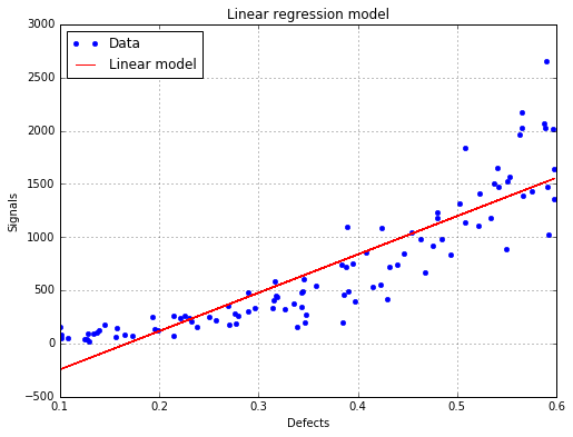
Intercept coefficient : -604.76
Slope coefficient : 3606.04
Standard error of the estimate : 291.47
Confidence interval on coefficients
Intercept coefficient : [-755.60, -453.91]
Slope coefficient : [3222.66, 3989.43]
Level : 0.95
Quality of regression
R2 (> 0.8): 0.78
--------------------------------------------------------------------------------
--------------------------------------------------------------------------------
Residuals analysis results
--------------------------------------------------------------------------------
Fitted distribution (uncensored) : Normal(mu = 6.01403e-13, sigma = 289.998)
Uncensored
Distribution fitting test
Kolmogorov p-value (> 0.05): 0.8
Normality test
Anderson Darling p-value (> 0.05): 0.07
Cramer Von Mises p-value (> 0.05): 0.09
Zero residual mean test
p-value (> 0.05): 1.0
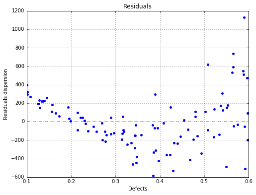
Homoskedasticity test (constant variance)
Breush Pagan p-value (> 0.05): 0.0
Harrison McCabe p-value (> 0.05): 0.2
Non autocorrelation test
Durbin Watson p-value (> 0.05): 0.99
--------------------------------------------------------------------------------
Warning : Some hypothesis tests failed : you may consider to use the Box Cox transformation.
Show graphs
Run analysis with Box Cox
analysis = otpod.UnivariateLinearModelAnalysis(defects, signals, boxCox=True)
Print results of the linear regression and all tests on the residuals
print(analysis.getResults())
--------------------------------------------------------------------------------
Linear model analysis results
--------------------------------------------------------------------------------
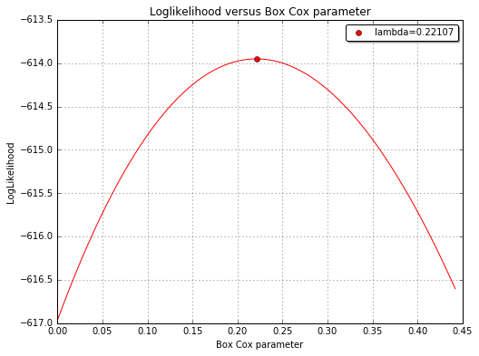
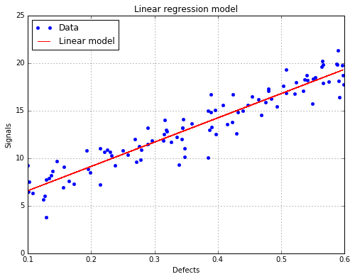
Box Cox parameter : 0.22
Uncensored
Intercept coefficient : 4.02
Slope coefficient : 25.55
Standard error of the estimate : 1.34
Confidence interval on coefficients
Intercept coefficient : [3.33, 4.72]
Slope coefficient : [23.80, 27.31]
Level : 0.95
Quality of regression
R2 (> 0.8): 0.89
--------------------------------------------------------------------------------
--------------------------------------------------------------------------------
Residuals analysis results
--------------------------------------------------------------------------------
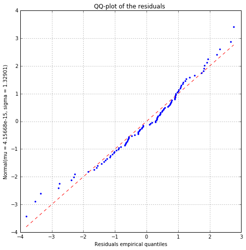
Fitted distribution (uncensored) : Normal(mu = 4.15668e-15, sigma = 1.32901)
Uncensored
Distribution fitting test
Kolmogorov p-value (> 0.05): 0.34
Normality test
Anderson Darling p-value (> 0.05): 0.06
Cramer Von Mises p-value (> 0.05): 0.07
Zero residual mean test
p-value (> 0.05): 1.0
Homoskedasticity test (constant variance)
Breush Pagan p-value (> 0.05): 0.65
Harrison McCabe p-value (> 0.05): 0.51
Non autocorrelation test
Durbin Watson p-value (> 0.05): 0.97
--------------------------------------------------------------------------------
Save all results in a csv file
analysis.saveResults('results.csv')
Show graphs
The linear regression model with data
fig, ax = analysis.drawLinearModel(name='figure/linearModel.png')
# The figure is saved as png file
fig.show()
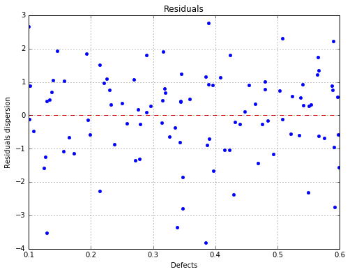
The residuals with respect to the defects
fig, ax = analysis.drawResiduals(name='figure/residuals.eps')
# The figure is saved as eps file
fig.show()
The fitted residuals distribution with the histogram
fig, ax = analysis.drawResidualsDistribution()
ax.set_ylim(ymax=0.45)
fig.show()
# The figure is saved after the changes
fig.savefig('figure/residualsDistribution.png', bbox_inches='tight')

The Box Cox likelihood with respect to the defect
fig, ax = analysis.drawBoxCoxLikelihood(name='figure/BoxCoxlikelihood.png')
fig.show()